
Planning Motion for a High DoF Robotic Arm
Published:
At first, this looked like a pathfinding problem with a more complicated object. There is a start pose, a goal pose, and a map with obstacles; surely I just needed to move the arm from one to the other. That intuition lasted until I tried to think about what a “position” meant for an arm with several joints.
The planner does not search over the pixels occupied by the arm. It searches over configurations: one angle for every joint. A point in this space is an entire pose of the arm, and a path is a sequence of poses that can be played back as continuous motion. Adding one joint adds another dimension to the search space, so the problem becomes difficult surprisingly quickly.

What I built
I implemented four sampling based planners in C++: RRT, RRT Connect, RRT*, and PRM. Each samples valid arm poses instead of discretizing the full configuration space.
How the planners work
All four planners operate on a configuration q = [θ₁, θ₂, …, θₙ], where each value is one joint angle. The distance between two configurations is the Euclidean distance between their angle vectors. When a planner proposes an edge from qₐ to qᵦ, I interpolate between those vectors and reject the entire edge if any intermediate arm pose is in collision.
The planners share the same edge validation routine:
VALID_EDGE(q_a, q_b)
    delta ← max_i |q_a[i] minus q_b[i]|
    steps ← max(2, ceil(delta / (pi / 90)))

    for k ← 0 to steps do
        t ← k / steps
        q ← (1 minus t)q_a + tq_b
        if ARM_IN_COLLISION(q) then
            return false
    return true
RRT: grow toward random samples
A Rapidly exploring Random Tree starts at the initial configuration. It samples a valid pose, finds the closest tree node, and moves one fixed size step toward the sample.
The tree is not explicitly told where unexplored space is. Random samples naturally pull it toward large empty regions, while branches that hit an obstacle stop growing. My implementation also tries to connect each newly added node to the goal. As soon as that edge is valid, it follows the parent pointers back to the start and returns the path.
RRT(q_start, q_goal)
    T ← tree containing q_start

    for iter ← 1 to MAX_ITERS do
        q_rand ← SAMPLE_FREE_CONFIGURATION()
        q_near ← NEAREST(T, q_rand)
        q_new  ← STEER(q_near, q_rand, STEP_SIZE)

        if VALID_EDGE(q_near, q_new) then
            T.ADD(q_new, parent = q_near)

            if VALID_EDGE(q_new, q_goal) then
                T.ADD(q_goal, parent = q_new)
                return TRACE_PARENTS(T, q_goal)

    return failure
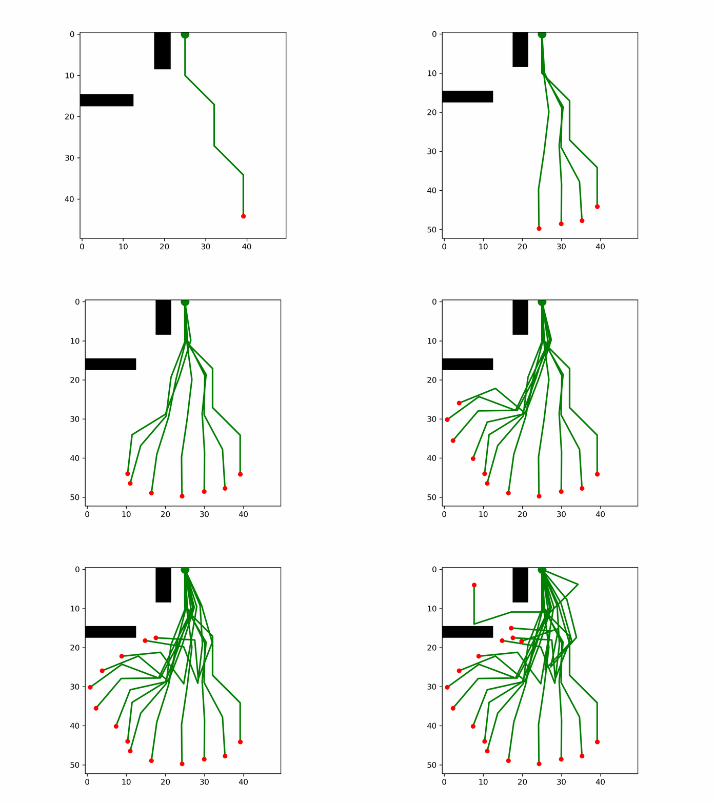
The playback contains seventeen poses and a visibly indirect sweep around the obstacles. That behavior matches the algorithm: RRT accepts the first valid connection to the goal and never revisits earlier parent choices to shorten the route.
RRT Connect: meet in the middle
RRT Connect keeps one tree at the start and another at the goal. One tree moves toward a random sample. The other repeatedly extends toward the new configuration until it reaches it or hits an obstacle. The trees then swap roles.
The two frontiers explore simultaneously and join their parent chains when they meet. The aggressive CONNECT step explains its speed in my tests.
RRT_CONNECT(q_start, q_goal)
    T_a ← tree containing q_start
    T_b ← tree containing q_goal

    for iter ← 1 to MAX_ITERS do
        q_rand ← SAMPLE_FREE_CONFIGURATION()
        status_a, q_new ← EXTEND(T_a, q_rand)

        if status_a != TRAPPED then
            status_b, q_meet ← CONNECT(T_b, q_new)

            if status_b = REACHED then
                path_a ← TRACE_PARENTS(T_a, q_new)
                path_b ← TRACE_PARENTS(T_b, q_meet)
                return STITCH(path_a, reverse(path_b))

        swap(T_a, T_b)

    return failure

CONNECT(T, q_target)
    repeat
        status, q_new ← EXTEND(T, q_target)
    until status != ADVANCED
    return status, q_new
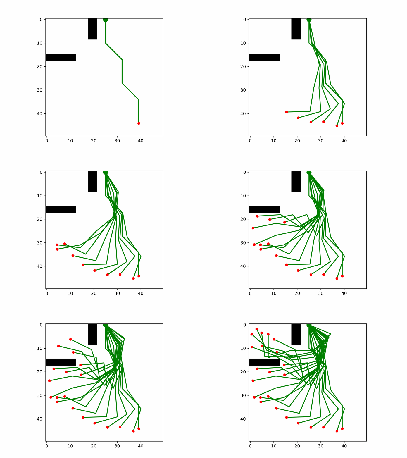
The sequence turns decisively around the obstacle and then advances through a dense run of nearby poses. This is consistent with the greedy connect operation: once one tree finds a useful direction, the other repeatedly extends toward it instead of returning to broad exploration. The result is fast, although the twenty four pose route is not the shortest one in the comparison.
RRT*: keep repairing the tree
RRT* chooses the valid parent that gives each new node the lowest total cost. It then rewires nearby nodes when routing them through the new node is cheaper.
This local repair improves path quality over time. My version caps the neighborhood at 20 nodes to limit collision checks.
RRT_STAR(q_start, q_goal)
    T ← tree containing q_start
    best_goal_parent ← none

    for iter ← 1 to MAX_ITERS do
        q_rand ← SAMPLE_FREE_CONFIGURATION()
        q_near ← NEAREST(T, q_rand)
        q_new  ← STEER(q_near, q_rand, STEP_SIZE)

        if not VALID_EDGE(q_near, q_new) then
            continue

        Q_near ← NEAR(T, q_new, radius, cap = 20)
        q_parent ← argmin over q in Q_near of
                    COST(q) + DISTANCE(q, q_new),
                    subject to VALID_EDGE(q, q_new)

        T.ADD(q_new, parent = q_parent)

        for each q in Q_near do
            candidate_cost ← COST(q_new) + DISTANCE(q_new, q)
            if candidate_cost < COST(q)
               and VALID_EDGE(q_new, q) then
                REWIRE(q, new_parent = q_new)

        if VALID_EDGE(q_new, q_goal)
           and COST(q_new) + DISTANCE(q_new, q_goal) improves best path then
            best_goal_parent ← q_new

    return TRACE_PARENTS(T, best_goal_parent) + q_goal
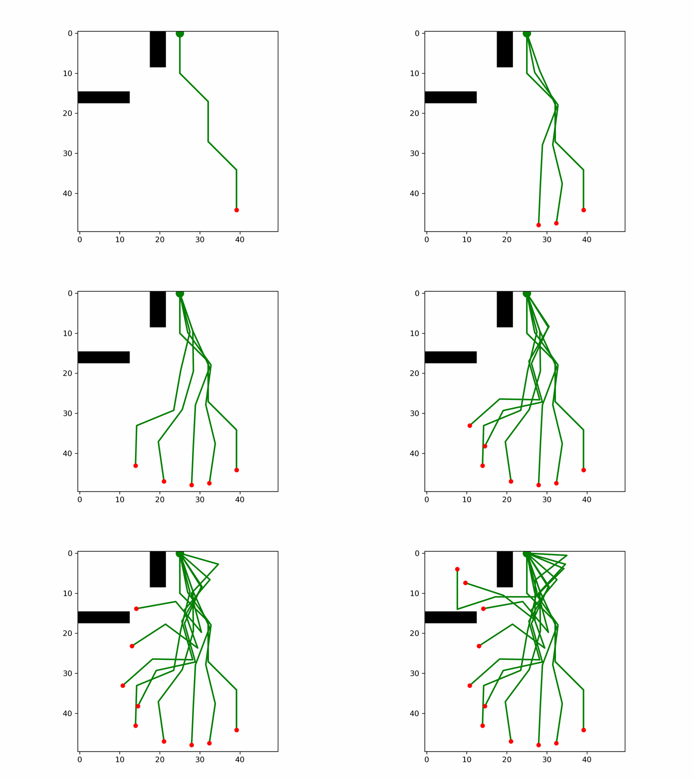
This playback reaches the same goal in eleven poses and avoids much of the broad sweep visible in RRT. The more direct motion is the visible consequence of parent selection and rewiring: feasible branches are not treated as final when a lower cost connection becomes available.
PRM: build a map of configuration space
A Probabilistic Roadmap samples 1,000 valid configurations and tries to connect each one to its 12 nearest neighbors. Dijkstra’s algorithm then finds the lowest cost route through the valid edges.
PRM(q_start, q_goal)
    V ← {q_start, q_goal}
    E ← empty set

    while |V| < NUM_SAMPLES + 2 do
        V.ADD(SAMPLE_FREE_CONFIGURATION())

    for each q in V do
        N_q ← K_NEAREST(V, q, K_NEIGHBORS)

        for each q_neighbor in N_q do
            if VALID_EDGE(q, q_neighbor) then
                E.ADD_UNDIRECTED_EDGE(
                    q,
                    q_neighbor,
                    weight = DISTANCE(q, q_neighbor)
                )

    return DIJKSTRA(V, E, q_start, q_goal)
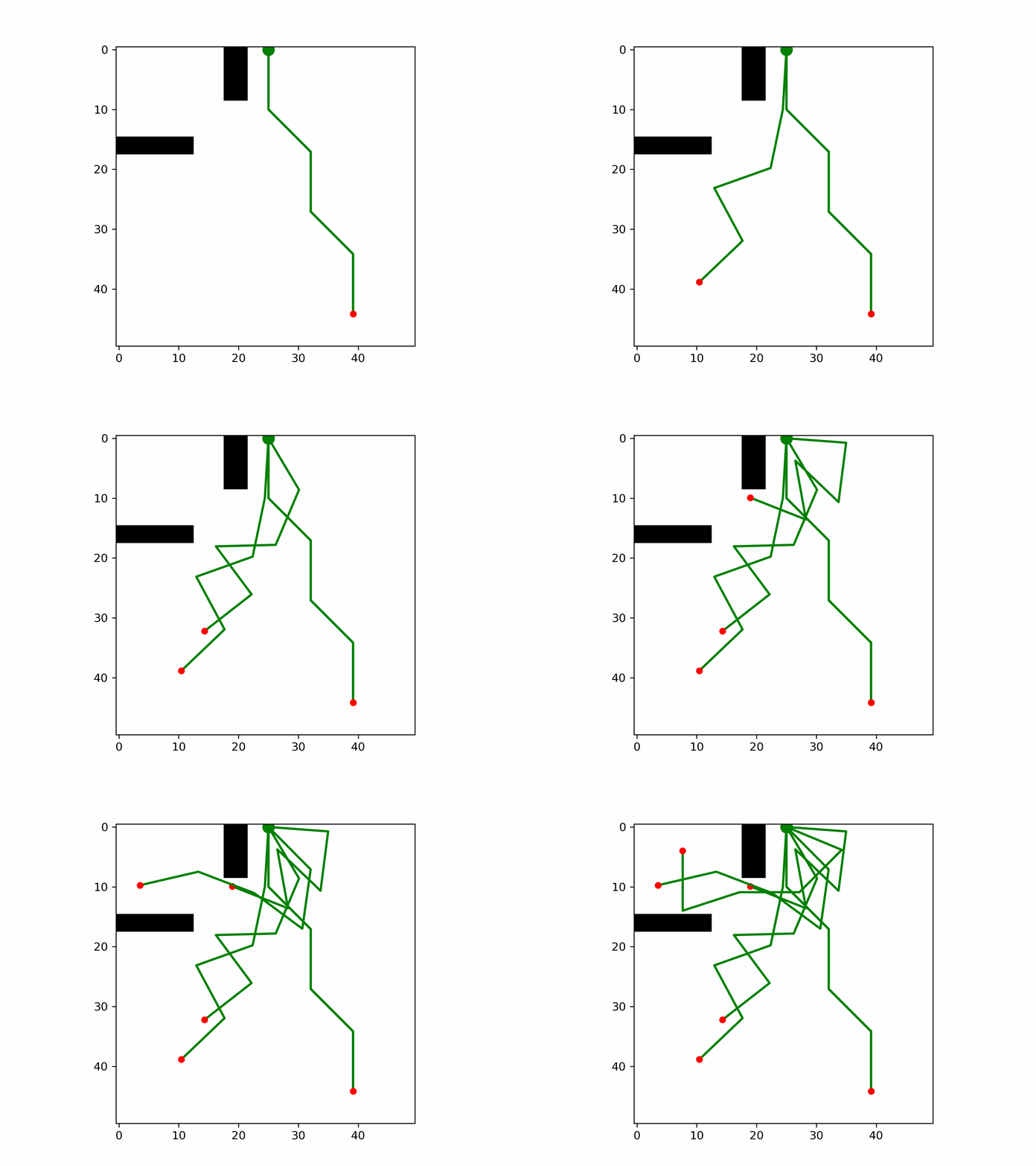
PRM uses only six playback poses, with sharper changes between some configurations. That sparse behavior follows from graph search over roadmap vertices: Dijkstra selects a low cost chain of prevalidated edges rather than growing a dense trajectory online. The expensive part happens before playback, when the roadmap is sampled and checked, but that work can support later queries on the same map.
The part that was harder than it looked
Collision checking was the first challenge. I used forward kinematics to recover each link segment and check it against the occupancy grid. Two valid configurations can still have an invalid motion between them, so I also checked interpolated poses along every proposed edge.
That check sits inside almost everything the planner does, so there is an uncomfortable tradeoff. Sample too sparsely and a collision can slip between two checks. Sample too densely and tree growth becomes slow. In my implementation, the number of checks depends on the largest change made by any joint, with poses checked at intervals of roughly two degrees.
Random samples become less useful as the number of joints grows, while nearest neighbor search becomes more expensive. I used a linear scan, which is simple but does not scale well.
RRT Connect required careful bookkeeping. Since the trees swap roles, path reconstruction can reverse the result or duplicate the meeting configuration.
The most difficult planner to reason about was RRT*. Choosing a cheaper parent for a new node was straightforward; rewiring existing nodes was not. A local parent change affects the meaning of the costs below it. My implementation updates the rewired node but does not propagate that reduction through all of its descendants. It worked for this project and produced good paths, but it is not the complete version I would want in a planning library.
Results
All four planners found valid solutions on the test cases. The benchmark summary from the repository is shown below.
| Planner | Success rate | Runtime (s) | Path cost | Relative result |
|---|---|---|---|---|
| RRT | 100% | 0.15 | 19.30 | Fast baseline |
| RRT Connect | 100% | 0.09 | 25.34 | Fastest |
| RRT* | 100% | 0.76 | 12.01 | Lowest cost path |
| PRM | 100% | 1.14 | 15.12 | Reusable roadmap |
Lower runtime and path cost are better. Path cost measures accumulated motion in joint angle space, not the physical distance traveled by the end effector.
| Planner | Search structure | Stops at first solution? | Main strength | Main cost |
|---|---|---|---|---|
| RRT | One tree from the start | Yes | Simple and quick to find a feasible route | Path can contain large detours |
| RRT Connect | Two alternating trees | Yes | Aggressively closes the gap | Fastest path is not necessarily short |
| RRT* | One rewired tree | No | Improves path cost as it samples | More neighbor searches and collision checks |
| PRM | Reusable undirected graph | No | Roadmap can serve repeated queries | Expensive construction and weak narrow passage coverage |
RRT Connect found a feasible path fastest. RRT* spent more time improving its tree and returned the lowest cost path. PRM was slowest for one query, but its roadmap can be reused.
I would not treat the timing differences as universal rankings. The maps are small, the planners are randomized, and the implementation choices matter. The result I trust more is the shape of the tradeoff: quickly finding a feasible path and deliberately searching for a better path are different goals.
What I took away from it
Before this project, I understood configuration space mostly as a diagram from lecture. Implementing the planners made it much more concrete. A motion that looks obvious in the workspace may be awkward in configuration space, while a strange-looking sequence of joint rotations may be exactly what lets the arm clear an obstacle.
The pseudocode for RRT fits in a few lines, but most of my work involved interpolation, collision checking, parent pointers, path ordering, and termination conditions. Those details made the difference between a valid planner and an outline of one.
Next, I would add a spatial index, improve angular wraparound, propagate descendant costs in RRT*, and evaluate more random seeds and narrow passages.